I Like Big Batches and I Cannot Lie

Understanding How to Train SoTA Embedding Models for Cheap

If you want to train the next best text embedding model, chances are you’ll need to use a large batch size. But naively scaling to the critical batch size requires lots of GPUs! But what happens if don’t have the compute budget to do so? GradCache allows you to fit large batch sizes with limited memory by decoupling the batch size from gradient calculation, the main source of memory.

We’ll explore why naive gradient accumulation doesn’t work and break down how GradCache works. We’ve used GradCache to train some of the embedding models at Nomic and I’ve found it essential for understanding the fundamentals of contrastive learning.

Big Batches are Better for Contrastive Learning

Contrastive representation learning trains a model to learn an embedding space such that similar data points are close to each other while dissimilar points are far away. Many modern embedding models, such as CLIP and OpenAI text-embedding-large, are trained with the InfoNCE loss. For a given batch size N of paired data¹, the model is trained to identify the positive pair amongst N-1 negative pairs in the batch. For example, each text caption is compared with every image in the batch. The loss forces all N-1 negative representations away from the caption and pull the positive image representation closer to the caption embedding.

Performance improves as you increase the batch size as you have more negative examples to compare against but doing so requires fitting the whole NxN similarity and activations into GPU memory.

But what happens if you don’t have enough memory to do so?

GradCache: Scaling Deep Contrastive Learning Batch Size under Memory Limited Setup

GradCache is a technique to reduce memory requirements by removing the backward pass’s dependency on the batch size. Let’s dig into how this works!

How Loss is Computed

The InfoNCE loss minimizes the categorical cross entropy loss between the positive pair and all other pairs in the batch. Each summation requires fitting the whole batch in memory.

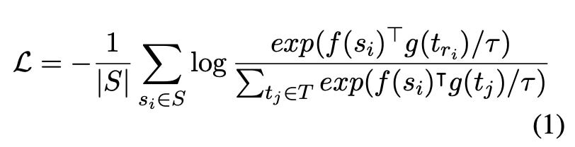
InfoNCE loss formulation used to train embedding models. Here f and g are models that output representations and S and T are the paired data points in the batch.

Why Can’t You Use Gradient Accumulation?

Naive gradient accumulation computes the loss and gradients in sub-batches then the model parameters are updated. In the case of your standard language modeling loss, the loss for each data point is independent of every other point in the batch! If you used gradient accumulation with the InfoNCE loss, you are only computing the negatives within the sub-batch.

Derivative of InfoNCE Loss

Let’s break down the derivatives of the InfoNCE loss. The models f and g are parameterized by Θ and Λ. Given the loss:

\(\mathcal{L} = -\frac{1}{|S|} \sum_{s_i \in S} \log \frac{\exp(f(s_i)^T g(t_{r_i})/\tau)}{\sum_{t_j \in T} \exp(f(s_i)^T g(t_j)/\tau)}\)

we want to derive the partial derivatives of the loss with respect to Θ and Λ:

\(\begin{align} \frac{\partial \mathcal{L}}{\partial \Theta} &= \sum_{s_i \in S} \frac{\partial \mathcal{L}}{\partial f(s_i)} \frac{\partial f(s_i)}{\partial \Theta} \\ \frac{\partial \mathcal{L}}{\partial \Lambda} &= \sum_{t_j \in T} \frac{\partial \mathcal{L}}{\partial g(t_j)} \frac{\partial g(t_j)}{\partial \Lambda} \end{align}\)

To make this more palatable, let’s work out the derivative for a single data point in S and T respectively

\(\begin{align} \mathcal{L}_i &= -\log \frac{\exp(f(s_i)^T g(t_{i}))}{\sum_{t_j \in T} \exp(f(s_i)^T g(t_j))} \\ \mathcal{L}_i &= -\log \frac{e^{a_i}}{\sum_{j} e^{a_j}} \\ &\text{where } a_i = f(s_i)^T g(t_{i})\\ \\ &= -a_i + \log(\sum_{j} e^{a_j}) \\ \frac{\partial \mathcal{L}_i}{\partial f(s_i)} &= \frac{\partial \mathcal{L}_i}{\partial a_i} \cdot \frac{\partial a_i}{\partial f(s_i)} + \sum_j \frac{\partial \mathcal{L}_i}{\partial a_j} \cdot \frac{\partial a_j}{\partial f(s_i)} \\ &= -g(t_i) + \sum_{t_j \in T}p_{ij} g(t_j) \tag{Appendix A} \\ &\text{where } p_{ij} = \frac{\exp(f(s_i)^T g(t_{j}))}{\sum_{t \in T} \exp(f(s_i)^T g(t))} \\ \\ \frac{\partial L}{\partial f(s_i)} &= -\frac{1}{|S|} \left(g(t_i) - \sum_{t_j \in T}p_{ij} g(t_j)\right)\\ \end{align}\)

We can interpret this partial derivative as how much we should pull the query representation f(s_i) toward the correct target representation g(t_i), and push it away from all other targets in the batch, weighted by their similarity.

Similarly, the partial derivative with respect to g(t_j) has a mirrored structure:

\(\begin{align} \frac{\partial \mathcal{L}_i}{\partial g(t_i)} &= \frac{\partial \mathcal{L}_i}{\partial a_i} \cdot \frac{\partial a_i}{\partial g(t_i)} + \sum_j \frac{\partial \mathcal{L}_i}{\partial a_j} \cdot \frac{\partial a_j}{\partial g(t_i)} \\ \frac{\partial \mathcal{L}}{\partial g(t_j)} &= -\frac{1}{|S|} \left( \sum_k \mathbf{1}[r_k = j] f(s_k) - \sum_{s_i \in S} p_{ij} f(s_i) \right) \end{align}\)

We push the target representation g(t_j) away from all queries that treat it as a negative (weighted by how similar they are), and pull it toward the corresponding query representation f(s_k) if it is the true positive match.

Looking at the partial derivatives, we can see we can’t use naive gradient accumulation as they rely on the full batch similarities.

So what can we do to reduce memory?

Breaking Apart

Remember the partial derivatives of the loss with respect to Θ and Λ?

\(\begin{align} \frac{\partial \mathcal{L}}{\partial \Theta} &= \sum_{s_i \in S} \frac{\partial \mathcal{L}}{\partial f(s_i)} \frac{\partial f(s_i)}{\partial \Theta} \\ \frac{\partial \mathcal{L}}{\partial \Lambda} &= \sum_{t_j \in T} \frac{\partial \mathcal{L}}{\partial g(t_j)} \frac{\partial g(t_j)}{\partial \Lambda} \end{align}\)

We can take advantage of two key properties of the gradient computation:

1. The loss gradient with respect to the representations (e.g., ∂L/∂f(s_i)) depends only on the numerical values of the representations and not on the encoder parameters Θ or Λ.

2. The gradient with respect to the encoder parameters (e.g., ∂L/∂Θ) depends only on ∂L/∂f(s_i) and the forward pass of f(s_i), but does not require the full batch.

This lets us avoid building a full end-to-end computational graph from input → encoder → embeddings → loss → gradient.

Instead, we can:

• Compute the representations without tracking gradients

• Compute the loss and the numerical gradients with respect to f(s_i) using the full batch.

• Re-run the forward pass of the encoder for each s_i and use the precomputed ∂L/∂f(s_i) to backpropagate and obtain ∂L/∂Θ.

This saves memory by avoiding the need to store encoder activations for the entire batch, while still enabling correct gradient computation.

GradCache can be thought of as a specialized case of gradient checkpointing. Training normally, you store all intermediate activations to compute gradients during the backward pass. Gradient checkpointing saves memory by discarding these activations and recomputing them during backward using a second forward pass.

GradCache takes this a step further for contrastive learning: it discards all activations for the encoder and recomputes only what's needed using precomputed gradients of the loss with respect to the embeddings. This means you avoid storing full-batch activations entirely.

Conclusion

In this article, we walked through why naive gradient accumulation doesn’t work for contrastive learning setups and how GradCache removes the batch dependency for gradient accumulation. GradCache allows you to scale to the critical batch size with limited hardware. Maybe you don’t need as much compute as you thought to train the next best embedding model!

Appendix

A.) Partial Derivative of LogSumExp

\(\begin{align} l &= \log\left(\sum_{j} \exp(x_j)\right) \\ \frac{\partial l}{\partial x_i} &= \frac{\partial l}{\partial x_i} \log\left(\sum_{j} \exp(x_j)\right) \\ &= \frac{\partial l}{\partial x_i} \log(z) \\ &\quad \text{where } z = \sum_{j} \exp(x_j) \\ &= \frac{\partial l}{\partial x_i}\frac{1}{\sum_{j} \exp(x_j)} * \exp(x_j)\\ &= \frac{\exp(x_i)}{\sum_{j} \exp(x_j)} \end{align}\)

1. Examples of this include question-answer pairs from search engines and images and their text captions. There is a lot of naturally occurring paired data; however not all of it is high quality!